-
Cisco IP Solution Center Traffic Engineering Management User Guide, 4.0
-
Index
-
About This Guide
-
Introduction to ISC TEM
-
Setting Up the Service
-
TE Network Discovery
-
TE Resource Management
-
Basic Tunnel Management
-
Advanced Primary Tunnel Management
-
Protection Planning
-
Traffic Admission
-
Administration
-
Task Monitoring
-
TE Topology
-
Traffic Engineering Management GUI
-
Warnings and Violations
-
Document Type Definition (DTD) File
-
 Feedback
Table Of Contents
Accessing the TE Topology Tool Page
Using the TE Topology Interface Applet
Using Highlighting and Attributes
Using AntiAlias, BackingStore, DoubleBuffer
TE Topology
The TE Topology tool provides a graphical view of the network set up through the Cisco IP Solution Center Traffic Engineering Management (ISC TEM) web client. It gives a graphical representation of the various network elements, including devices, links, and tunnels.
This section describes how to use the topology tool. A definition of fields and buttons in the topology GUI is found in TE Topology in "Traffic Engineering Management GUI".
This chapter contains the following sections:
•
Accessing the TE Topology Tool Page
•
Overview
The TE Topology tool can be activated from various locations within ISC. However, in this user guide the TE Topology tool is assumed to be accessed from the Traffic Engineering Management Services page.
The TE Topology tool is used to visualize the TE network based on the data contained in the repository. To that end, it provides a number of ways of manipulating the display, for example by applying algorithms to the graph layout, importing maps, and so on.
The tool is accessed from a TE Topology Interface Applet that displays the TE topology through a Java applet within the browser.
Accessing the TE Topology Tool Page
The TE Topology tool is accessed as follows:
Step 1
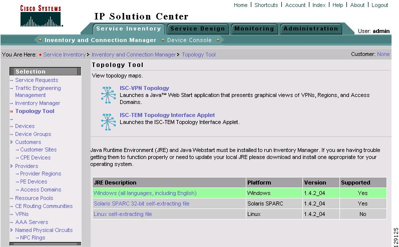
The Topology Tool window in Figure 11-1 appears.
Figure 11-1 Topology Tool
For a detailed description of the Topology Tool page, see Cisco IP Solution Center Infrastructure Reference, 4.0.
Step 2
Using the TE Topology Interface Applet
The TE Topology Interface Applet (Topology Applet) provides a means of visualizing the network and tunnels present in the network. The web-based GUI is the primary means of visualizing the network information. The Topology Applet simply augments the web-based GUI to provide a different presentation format to the user.
The features offered through the Topology Applet are:
•
•
•
•
•
To access the Topology Applet, use the following steps:
Step 1
Step 2
The security warning window in Figure 11-2 appears.
Figure 11-2 Security Warning
Step 3
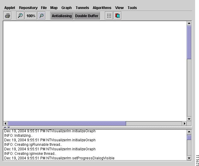
The Topology Display applet window in Figure 11-3 appears.
Figure 11-3 Topology Display Applet
For an explanation of the various window elements in all the menus of the Topology Display, see Topology Display Window.
Display/Save Layout
Use the two operations in the Repository menu, Layout Graph and Save Graph Layout, to display or save the current layout of the network graph.
Prior to generating the graph layout, the coordinates must be set on each of the network devices. Otherwise, the graph will have a random layout.
•
•
Using Maps
You can associate a map with each view. Currently, the topology viewer only supports maps in the Environmental Systems Research Institute, Inc. (ESRI) shape format. The following sections describe how to load maps and selectively view map layers and data associated with each map.
The map features are accessed from the Map menu in the Topology window.
To access the Map menu, use the following steps:
Step 1
Step 2
Step 3
Figure 11-4 The Map Menu
From the Map menu, you can either load or clear (remove) maps as described in the following.
Loading a map
You might wish to set a background map showing the physical locations of the displayed devices. To load a map, use the following steps:
Step 1
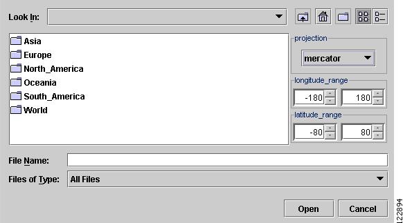
Providing the web map server is running, the Load Map window appears (see Figure 11-5).
Figure 11-5 Load Map
For an explanation of the various window elements , see Load Map.
Step 2
The right-hand side of the window contains a small control panel, which allows you to select the projection in which a map is shown. A map projection is a projection which maps a sphere onto a plane. Typical projections are Mercator, Lambert, and Stereographic.
For more information on projections, consult the Map Projections section of Eric Weisstein's World of Mathematics at:
http://mathworld.wolfram.com/topics/MapProjections.html
For each projection, you can also select the region of the map to be shown. In most cases, the predefined values should be sufficient. The top level of the file hierarchy should contain folders for all major regions, such as Asia, Europe, North America, Oceania, and so on.
If desired, make changes to the settings in the Longitude Range and Latitude Range fields.
Step 3
Each folder can contain either complete maps or folders for countries. Each map is clearly distinguished with the Map icon.
Step 4
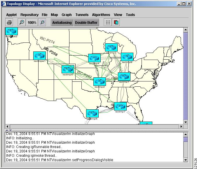
Selecting the map file and clicking the Open button starts loading it. Maps can consist of several components and thus a progress dialog is shown informing you which part of the map file is loaded.
A map similar to the one in Figure 11-6 appears.
Figure 11-6 Loaded Map
Step 5
Adding new maps
You might need to add your own maps to the selection of maps available to the Topology Tool. This is done by placing a map file in the $ISC_HOME/resources/webserver/tomcat/webapps/ipsc-maps/data directory or a subdirectory thereof within the ISC installation. To make this example more accessible, assume that you wish to add a map of Toowong, a suburb of Brisbane, the capital of Queensland. The first step to do so is to obtain maps from a map vendor. All maps must be in the ESRI shape file format (see ESRI shapefile technical description). In addition, a data file can accompany each shape file. Data files contain information about objects and the corresponding shapes are contained within the shape file. Let us assume that the vendor provided four files:
•
•
•
•
We have to create a .map file that informs the TE Topology tool about layers of the map. In this case we have two layers: a city and a street layer. The map file, say, Toowong.map, would thus have the following contents:
toowong_citytoowong_streetIt lists all layers that create a map of Toowong. The order is important, as the first file forms the background layer, with other layers placed on top of the preceding layers.
Having obtained shape and data files and having written the map file, decide on its location. As mentioned, Toowong is a suburb of Brisbane, located in Queensland, Australia. All map files must be located in or under the $ISC_HOME/resources/webserver/tomcat/webapps/ipsc-maps/data directory. Since by default this directory contains a directory called Oceania intended for all maps from that region, simply create a path Australia/Queensland/Brisbane under the directory Oceania. Next, place all five files in this location. Once this is done, the map is automatically accessible to the topology viewer.
Clearing Maps
To clear the active map, select Map > Clear (see Figure 11-3 and Figure 11-4).
Use this feature to clear (remove) the active map to leave only nodes and links in the corresponding network.
Using Highlighting and Attributes
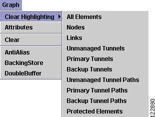
The Graph menu, shown in Figure 11-7, provides access to a range of tools to manage and manipulate graphs.
Figure 11-7 Graph Menu
For an explanation of the various menu items, see the following sections as well as Graph.
Use the JavaServer Pages (to pagesto) to look at the list of nodes, links, and tunnels. From the JSP pages, select the display button at the bottom of the window to highlight elements.
The tools in the Graph menu serve to modify the appearance of the topology.
These are described in the following sections.
Clear Highlighting
Clear Highlighting serves to remove highlighting from specific elements as listed in its submenus. For a description of the individual entries, see Graph.
Add/Modify Attributes
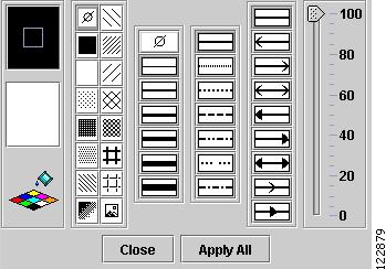
When you select Attributes from the Graph menu, the Graphic Attributes window in Figure 11-8 appears.
Figure 11-8 Graphic Attributes
The Add/Modify Attributes tool is used as follows:
Step 1
Step 2
Step 3
Note
Clear Current Graph Layout
Use the Clear function in the Graph menu to remove the topology graph from the current view.
Although this is also achieved with Layout Graph in the Repository menu, Layout Graph re-creates the graph last saved in the repository in addition to clearing the graph.
Using AntiAlias, BackingStore, DoubleBuffer
AntiAlias, found in the Graph menu, is used to create smoother lines and a more pleasant appearance at the expense of performance.
BackingStore allows graphics content to be automatically saved when moved to the background and regenerated when returned to the foreground. This helps avoid superfluous refreshing.
DoubleBuffer enables double buffering for dragging elements on the graph.
Using Algorithms
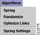
In the Algorithms menu, shown in Figure 11-9, various algorithms can be used to enhance and otherwise alter the graph layout.
Note
Spring is a graph layout algorithm that optimizes the graph layout based on weights.
Randomize rearranges the nodes in the current topology layout at random.
If there are overlapping links, the layout can be optimized by selecting Optimize Links.
Figure 11-9 Algorithms Menu
For further explanation of the Algorithms menu, see Algorithms Menu.
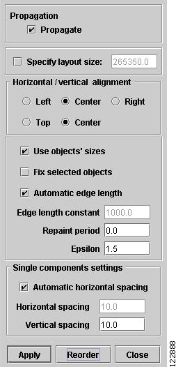
The spring settings are used to enhance the appearance of the topology display according to user preferences. When selecting Spring Settings, the Spring Settings window in Figure 11-10 appears.
Figure 11-10 Spring Settings
For an explanation of the various fields in the Spring Settings window, see Algorithms.