-
Cisco Wireless Control System Configuration Guide, Release 5.1
-
Preface
-
Chapter 1: Overview
-
Chapter 2: Getting Started
-
Chapter 3: Configuring Security Solutions
-
Chapter 4: Performing System Tasks
-
Chapter 5: Adding and Using Maps
-
Chapter 6: Monitoring Wireless Devices
-
Chapter 7: Managing WCS User Accounts
-
Chapter 8: Configuring Mobility Groups
-
Chapter 9: Configuring Access Points
-
Chapter 10: Configuring Controllers and Switches
-
Chapter 11: Using Templates
-
Chapter 12: Performing Maintenance Operations
-
Chapter 13: Configuring Hybrid REAP
-
Chapter 14: Alarms and Events
-
Chapter 15: Running Reports
-
Chapter 16: Administrative Tasks
-
Chapter 17: Virtual Domains
-
Chapter 18: Google Earth Maps
-
Appendix A: Troubleshooting and Best Practices
-
Appendix B: WCS and End User Licenses
-
Appendix C: Conversion of a WLSE Autonomous Deployment to a WCS Controller Deployment
-
Index of Cisco Wireless Control System Configuration Guide, Version 5.1
-
 Feedback
Table Of Contents
Adding a Building to a Campus Map
Enabling Location Presence on a Location Server
Adding and Enhancing Floor Plans
Adding Floor Plans to a Campus Building
Adding Floor Plans to a Standalone Building
Using the Map Editor to Enhance Floor Plans
Using the Map Editor to Draw Polygon Areas
Using Planning Mode to Calculate Access Point Requirements
Changing Access Point Positions by Importing and Exporting a File
Using Chokepoints to Enhance Tag Location Reporting
Adding Chokepoints to the WCS Database and Map
Removing Chokepoints from the WCS Database and Map
Monitoring Channels on a Floor Map
Monitoring Transmit Power Levels on a Floor Map
Monitoring Coverage Holes on a Floor Map
Monitoring Clients on a Floor Map
Importing or Exporting WLSE Map Data
Creating and Applying Calibration Models
Analyzing Element Location Accuracy Using Testpoints
Assigning Testpoints to a Selected Area
Using the Accuracy Tool to Conduct Accuracy Testing
Using Scheduled Accuracy Testing to Verify Accuracy of Current Location
Using On-Demand Accuracy Testing to Test Location Accuracy
Adding and Using Maps
This chapter describes how to add maps to the Cisco WCS database and use them to monitor your wireless LAN. It contains these sections:
•
Using Chokepoints to Enhance Tag Location Reporting
•
•
•
•
Creating Maps
With the Cisco WCS database, you can add maps and view your managed system on realistic campus, building, and floor map maps. Follow the instructions in the sections below to add a campus, buildings, outdoor areas, floor plans, and access points to maps in the Cisco WCS database:
Adding a Campus
Follow these steps to add a single campus map to the Cisco WCS database.
Step 1
Note
Step 2
Step 3
Step 4
Step 5
Step 6
Step 7
Step 8
Note
Step 9
Adding Buildings
You can add buildings to the Cisco WCS database regardless of whether you have added campus maps to the database. This section explains how to add a building to a campus map or a standalone building to the Cisco WCS database.
Adding a Building to a Campus Map
Follow these steps to add a building to a campus map in the Cisco WCS database.
Step 1
Step 2
Step 3
Step 4
a.
b.
c.
d.
Tip
e.
f.
Note
g.
Note
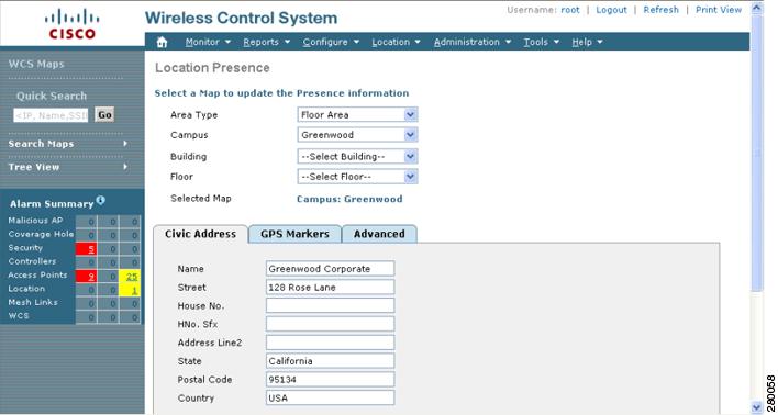
Step 5
a.
Figure 5-1 Location Presence Window
b.
–
–
–
Note
Note
c.
Step 6
Adding a Standalone Building
Follow these steps to add a standalone building to the Cisco WCS database.
Step 1
Step 2
Step 3
a.
b.
Note
c.
d.
Note
e.
Step 4
a.
b.
–
–
–
Note
Note
c.
Step 5
Adding Outdoor Areas
Follow these steps to add an outdoor area to a campus map.
Note
Step 1
Note
Step 2
Step 3
Step 4
Step 5
a.
b.
c.
d.
Tip
e.
f.
g.
Note
Step 6
a.
b.
–
–
–
Note
Note
c.
Step 7
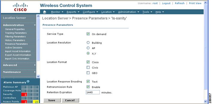
Enabling Location Presence on a Location Server
Follow these steps to enable and configure location presence on a location server. When enabled, the location server is capable of providing any requesting Cisco Compatible Extension v5 client with its location.
Note
Step 1
Step 2
Figure 5-2 Location Server > Presence Parameters Window
Step 3
Step 4
a.
–
b.
–
c.
–
Step 5
a.
b.
c.
Step 6
Step 7
Step 8
Step 9
Searching Maps
Use the controls in the left sidebar to create and save custom searches:
•
•
•
•
You can configure the following parameters in the Search Maps window:
•
•
•
•
•
After you click GO, the map search results window appears:
Finding Coverage Holes
Coverage holes are areas where clients cannot receive a signal from the wireless network. The Cisco Unified Wireless Network Solution radio resource management (RRM) identifies these coverage hole areas and reports them to WCS, enabling the IT manager to fill holes based on user demand. Follow these steps to find coverage holes on your wireless LAN.
Step 1
Step 2
Step 3
Step 4
Adding and Enhancing Floor Plans
This section explains how to add floor plans to either a campus building or a standalone building in the Cisco WCS database. It also provides instructions on using the WCS map editor to enhance floor plans that you have created and the WCS planning mode to calculate the number of access points required to cover an area.
Adding Floor Plans to a Campus Building
After you add a building to a campus map, you can add individual floor plan and basement maps to the building. Follow these steps to add floor plans to a campus building.
Step 1
Note
Step 2
Step 3
Step 4
Step 5
Note
Step 6
Step 7
Step 8
a.
b.
c.
d.
e.
f.
g.
Note
h.
i.
j.
Note
k.
Tip
l.
Note
Step 9
Note
Adding Floor Plans to a Standalone Building
After you have added a standalone building to the Cisco WCS database, you can add individual floor plan maps to the building. Follow these steps to add floor plans to a standalone building.
Step 1
Note
Step 2
Step 3
Step 4
Step 5
Step 6
a.
b.
c.
d.
e.
f.
g.
Note
h.
Note
i.
j.
Note
k.
Tip
l.
Step 7
Note
Using the Map Editor to Enhance Floor Plans
You can use the WCS map editor to define, draw, and enhance floor plan information. The map editor enables you to create obstacles so that they can be taken into consideration when computing RF prediction heat maps for access points. You can also add coverage areas for location appliances that locate clients and tags in that particular area. Follow these general guidelines to use the map editor.
General Notes and Guidelines for Using the Map Editor
Consider the following when modifying a building or floor map using the map editor.
•
–
•
–
•
–
•
Follow these steps to use the map editor.
Step 1
Step 2
Step 3
Step 4
Step 5
Step 6
Step 7
Step 8
Step 9
Step 10
Step 11
Step 12
Step 13
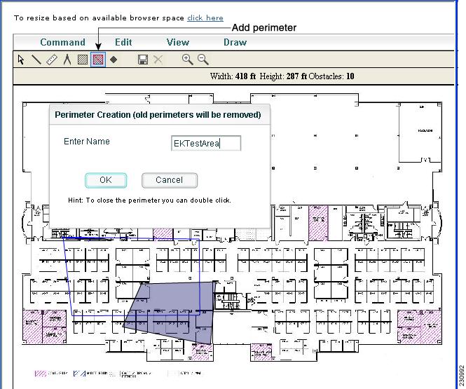
Using the Map Editor to Draw Polygon Areas
If you have a building that is non-rectangular or you want to mark a non-rectangular area within a floor, you can use the map editor to draw a polygon-shaped area.
Step 1
Step 2
Step 3
Step 4
Step 5
A pop-up window appears.
Note
Figure 5-3 Map Editor Page
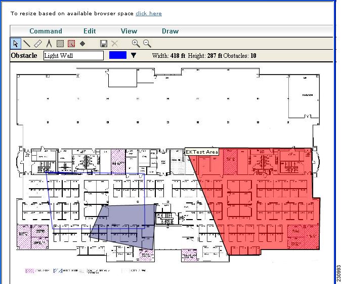
Step 6
A drawing tool appears.
Step 7
•
•
•
Figure 5-4 Polygon Area
Step 8
Step 9
Note
Step 10
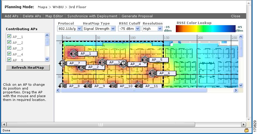
Using Planning Mode to Calculate Access Point Requirements
The WCS planning mode enables you to calculate the number of access points required to cover an area by placing fictitious access points on a map and allowing you to view the coverage area. Based on the throughput specified for each protocol (802.11a/n or 802.11b/g/n), planning mode calculates the total number of access points required to provide optimum coverage in your network. You can calculate the recommended number and location of access points based on the following criteria:
•
•
•
•
To calculate the recommended number and placement of access points for a given deployment, follow these steps:
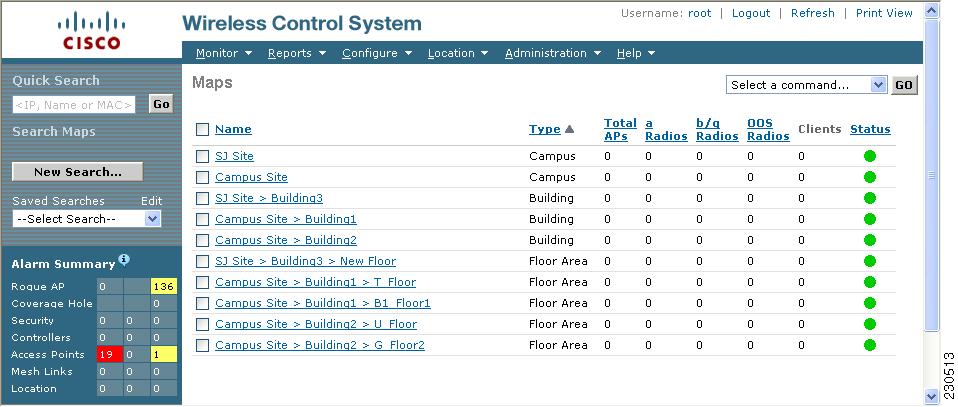
Step 1
The window appears (see Figure 5-5).
Figure 5-5 Monitor > Maps Page
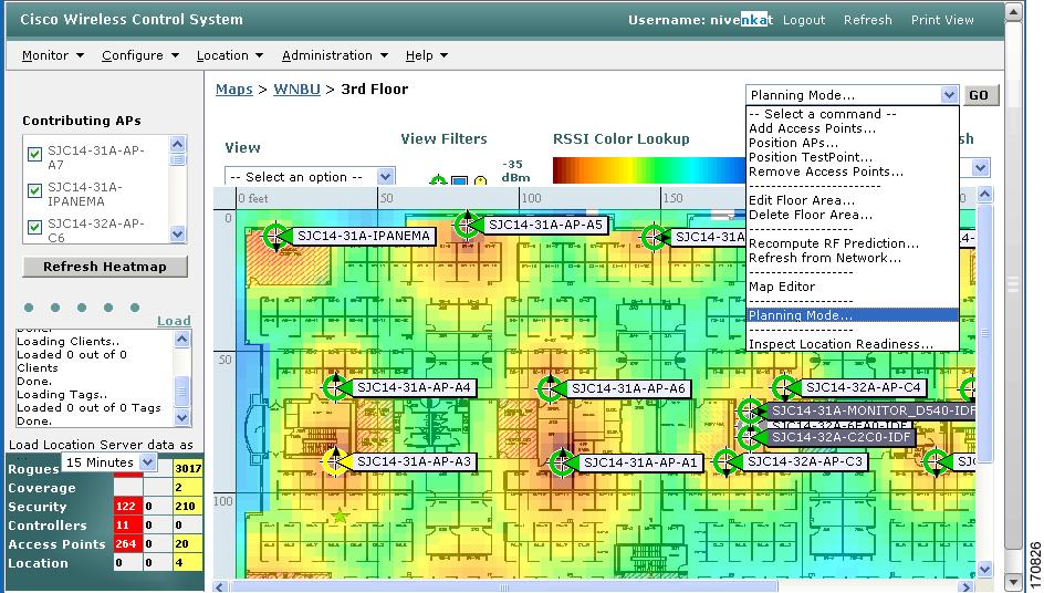
Step 2
A color-coded map appears showing placement of all installed elements (access points, clients, tags) and their relative signal strength (see Figure 5-6).
Figure 5-6 Selected Floor Area Showing Current Access Point Assignments
Step 3
Step 4
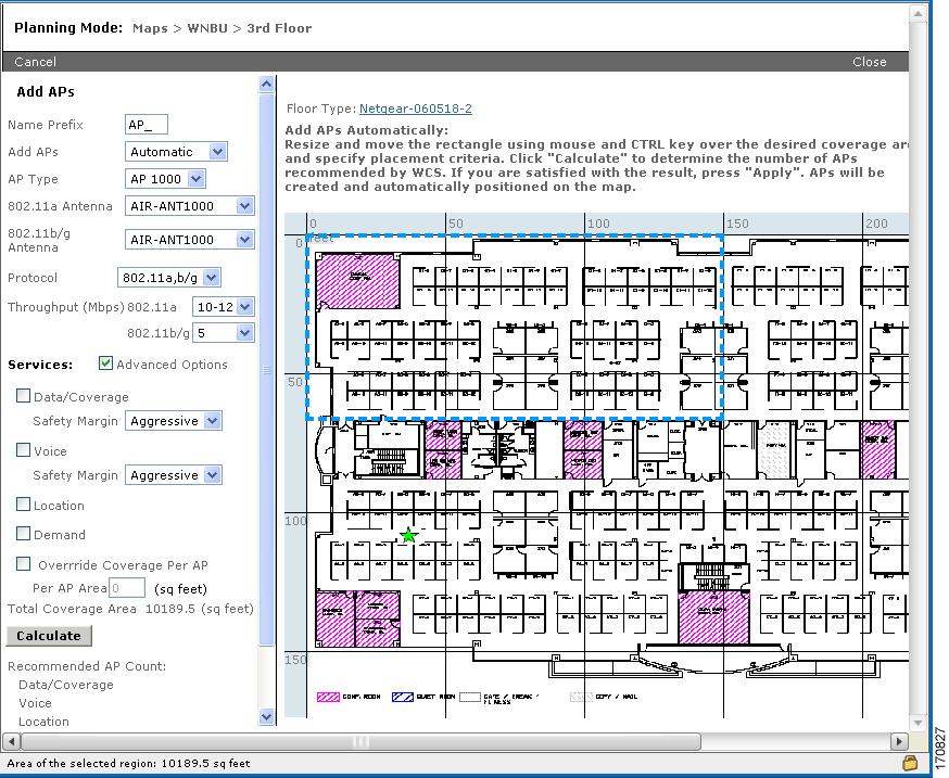
Step 5
Note
Figure 5-7 Add APs Page
Step 6
Step 7
Step 8
Step 9
Note
Note
Table 5-2 Definition of Service Options
Table 5-3 Definition of Advanced Options
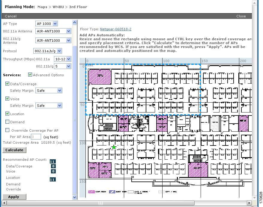
Step 10
The recommended number of access points given the selected services appears (see Figure 5-8).
Figure 5-8 Recommended Number of Access Points Given Selected Services and Parameters
Note
Note
Step 11
Figure 5-9 Recommended Access Point Deployment Given Selected Services and Parameters
Step 12
Inspect VoWLAN Location Readiness
The Inspect Location Readiness feature is a distance-based predictive tool that can point out problem areas with access point placement.
The Inspect Location Readiness tool:
•
•
•
A point is defined as "location-ready" if the following is true:
•
•
•
To access the Inspect Location Readiness tool, follow these steps:
Step 1
Step 2
Step 3
Inspect VoWLAN Readiness
Voice readiness tool (the VoWLAN Readiness tool) allows you to verify that the RF coverage is sufficient for your voice needs. This tool verifies RSSI levels after access points have been installed.
To access the VoWLAN Readiness Tool (VRT), follow these steps:
Step 1
Step 2
Step 3
Step 4
Note
Step 5
•
•
–
–
Step 6
•
•
•
Troubleshooting Voice RF Coverage Issues
Perform the following to troubleshoot voice RF coverage issues:
•
•
•
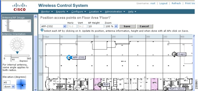
Adding Access Points
After you add the .PNG, .JPG, .JPEG, or .GIF format floor plan and outdoor area maps to the Cisco WCS database, you can position lightweight access point icons on the maps to show where they are installed in the buildings. Follow these steps to add access points to floor plan and outdoor area maps.
Step 1
Step 2
Step 3
Step 4
Note
Step 5
Step 6
Figure 5-10 Antenna Sidebar
Note
•
•
•
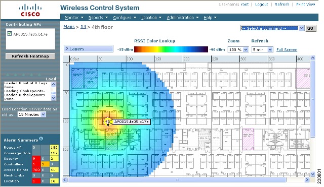
Step 7
Note
Figure 5-11 RF Prediction Heat Map
Placing Access Points
To determine the optimum location of all devices in the wireless LAN coverage areas, you need to consider the access point density and location.
Ensure that no fewer than 3 access points, and preferably 4 or 5, provide coverage to every area where device location is required. The more access points that detect a device, the better. This high level guideline translates into the following best practices, ordered by priority:
1.
2.
Note
Following these guidelines makes it more likely that access points will detect tracked devices. Rarely do two physical environments have the same RF characteristics. Users may need to adjust those parameters to their specific environment and requirements.
Note
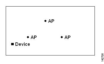
Guidelines for Placing Access Points
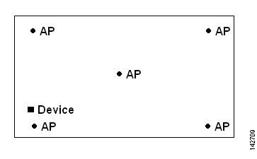
Follow these rules for placing access points accurately:
1.
Figure 5-12 Access Points Clustered Together
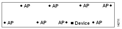
2.
Figure 5-13 Improved Location Accuracy by Increasing Density
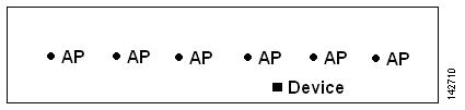
3.
Figure 5-14 Refrain From Straight Line Placement
Although the design in Figure 5-14 may provide enough access point density for high bandwidth applications, location suffers because each access point's view of a single device is not varied enough; therefore, location is difficult to determine.
4.
Figure 5-15 Improved Location Accuracy by Staggering Around Perimeter
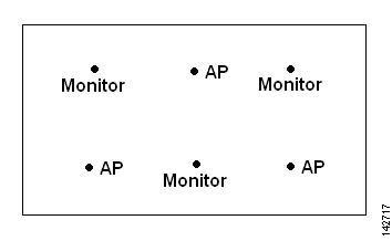
5.
Less dense wireless LAN installations, such as voice networks, find their location accuracy greatly increased by the addition and proper placement of monitor access points (see Figure 5-16).
Figure 5-16 Less Dense Wireless LAN Installations
6.
Creating a Network Design
After access points have been installed and have joined a controller, and WCS has been configured to manage the controllers, set up a network design. A network design is a representation within WCS of the physical placement of access points throughout facilities. A hierarchy of a single campus, the buildings that comprise that campus, and the floors of each building constitute a single network design. These steps assume that the location appliance is set to poll the controllers in that network, as well as be configured to synchronize with that specific network design, in order to track devices in that environment. The concept and steps to perform synchronization between WCS and the location appliance are explained in the "Importing the Location Appliance into WCS" section on page 12-7.
Designing a Network
Follow these steps to design a network.
Step 1
Note
Step 2
Step 3
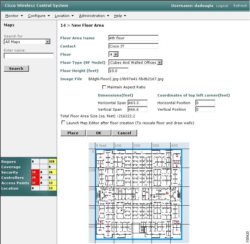
Figure 5-17 Creating a New Network Design
Step 4
Step 5
Step 6
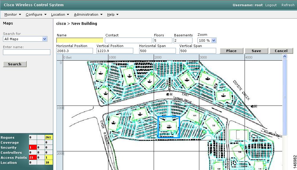
You should uncheck the Maintain Aspect Ratio check box if you want to override this automatic adjustment. You could then adjust both span values to match the real world campus dimensions.Step 7
Step 8
Step 9
Figure 5-18 New Building
Step 10
Step 11
Figure 5-19 Repositioning Building Highlighted in Blue
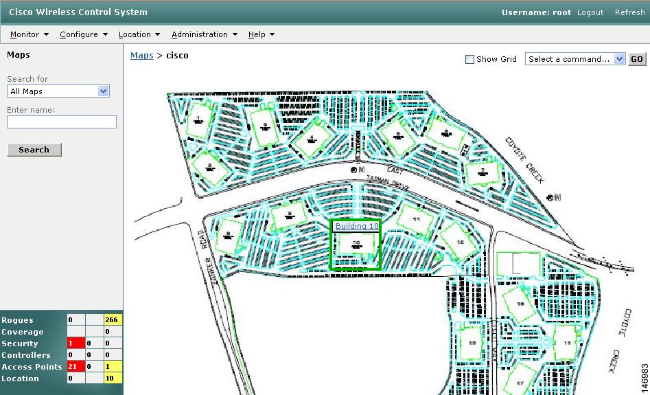
Step 12
Figure 5-20 Newly Created Building Highlighted in Green
Step 13
Step 14
Step 15
Step 16
Step 17
Note
Step 18
Figure 5-21 Repositioning Using Numerical Value Fields
Step 19
Step 20
Step 21
Step 22
Step 23
Note
Step 24
Changing Access Point Positions by Importing and Exporting a File
You can change an access point position by importing or exporting a file. The file contains only the lines describing the access point you want to move. This option takes less time than manually changing multiple access point positions. Follow these steps to change access point positions using the importing or exporting of a file.
Step 1
Step 2
Step 3
Step 4
Step 5
Note
Note
Step 6
Using Chokepoints to Enhance Tag Location Reporting
Installation of chokepoints provides enhanced location information for RFID tags. When an active Cisco Compatible Extensions version 1 compliant RFID tag enters the range of a chokepoint, it is stimulated by the chokepoint. The MAC address of this chokepoint is then included in the next beacon sent by the stimulated tag. All access points that detect this tag beacon then forward the information to the controller and location appliance.
Using chokepoints in conjunction with active compatible extensions compliant tags provides immediate location information on a tag and its asset. When a Cisco Compatible Extension's tag moves out of the range of a chokepoint, its subsequent beacon frames do not contain any identifying chokepoint information. Location determination of the tag defaults to the standard calculation methods based on RSSIs reported by the access point associated with the tag.
Adding Chokepoints to the WCS Database and Map
Chokepoints are installed and configured as recommended by the Chokepoint vendor. After the chokepoint installation is complete and operational, the chokepoint is added to WCS and placed on floor maps. They are forwarded to the location server during synchronization.
Follow these steps to add a chokepoint to the WCS database and appropriate map:
Step 1
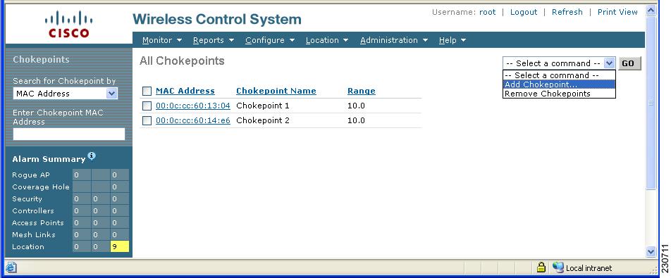
The All Chokepoints summary window appears (see Figure 5-22).
Figure 5-22 Configure > Chokepoints
Step 2
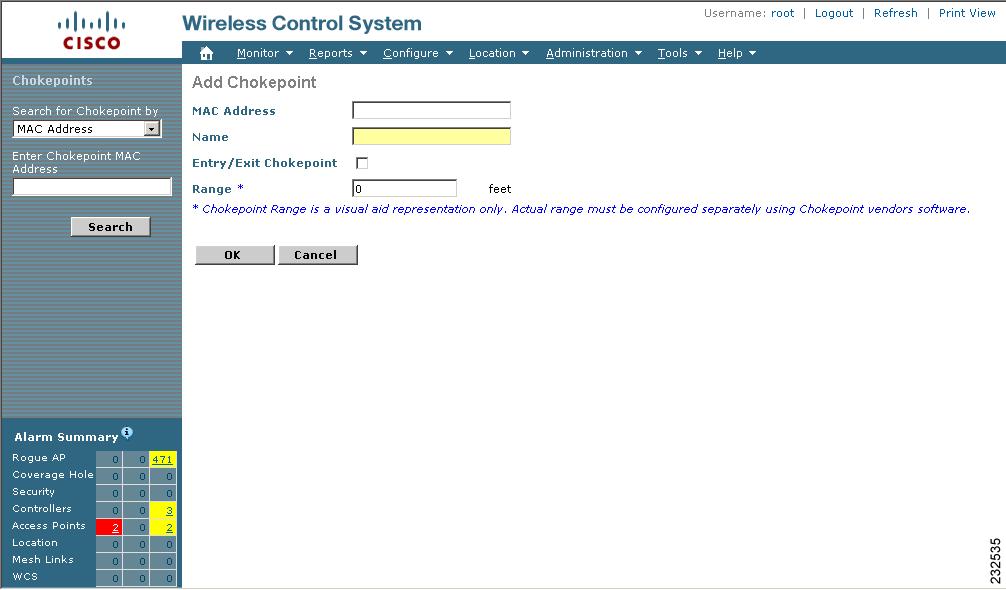
The Add Chokepoint entry window appears (see Figure 5-23).
Figure 5-23 Add Chokepoint Configuration Page
Step 3
Note
Step 4
Step 5
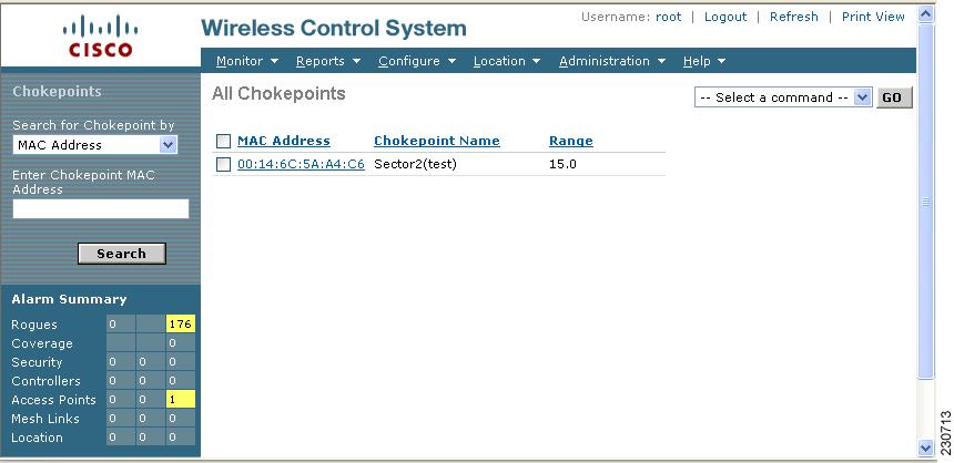
The All Chokepoints summary page appears with the new chokepoint entry listed (Figure 5-24).
Figure 5-24 All Chokepoints Summary Page
Note
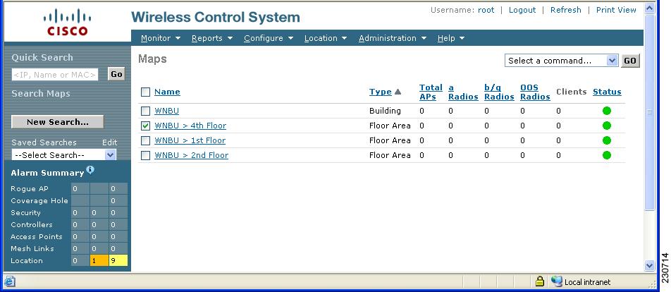
Step 6
Figure 5-25 Monitor > Maps
Step 7
Figure 5-26 Selected Floor Map
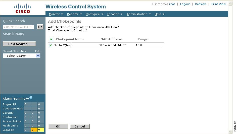
Step 8
The Add Chokepoints summary page appears (see Figure 5-27).
Note
Figure 5-27 Add Chokepoints Summary Page
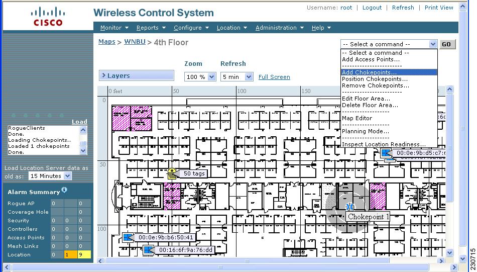
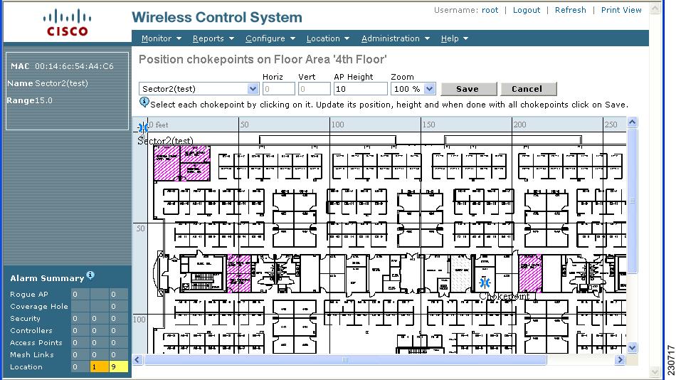
Step 9
A map appears with a chokepoint icon located in the top-left hand corner (Figure 5-28). You are now ready to place the chokepoint on the map.
Figure 5-28 Map for Positioning Chokepoint
Step 10
Figure 5-29 Chokepoint Icon Positioned on the Floor Map
Note
Step 11
You are returned to the floor map and the added chokepoint appears on the map.
Note
Figure 5-30 New Chokepoint Appears on Floor Map
Note
Note
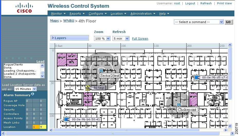
Step 12
The chokepoint appears on the map (Figure 5-31).
Figure 5-31 Display Chokepoints on Map
Step 13
Note
Removing Chokepoints from the WCS Database and Map
You can remove one or multiple chokepoints at a time.
Follow these steps to delete a chokepoint.
Step 1
Step 2
Step 3
Step 4
You are returned to the All Chokepoints page. A message confirming deletion of the chokepoint appears. The deleted chokepoint(s) is no longer listed on the page.
Monitoring Chokepoints
Chokepoints are installed and configured as recommended by the chokepoint vendor. Chokepoints are added to WCS and placed on floor maps, and then they are pushed to the location server during synchronization. Choose Monitor > Chokepoints to display a list of found chokepoints. Clicking the link under Map Location for a particular chokepoint displays a map that shows the location of the chokepoint. The following parameters are displayed:
•
•
•
•
•
Monitoring Maps
This section describes how to use maps to monitor your wireless LANs and predict coverage. You can use maps to do the following:
•
•
•
•
In preparation for monitoring your wireless LANs, familiar yourself with the various refresh options for a map.
•
Note
•
•
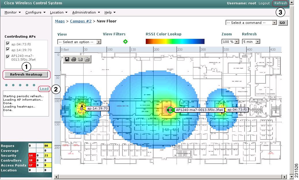
Figure 5-32 Monitoring Maps
Note
Monitoring Predicted Coverage
Follow these steps to monitor the predicted wireless LAN coverage on a map.
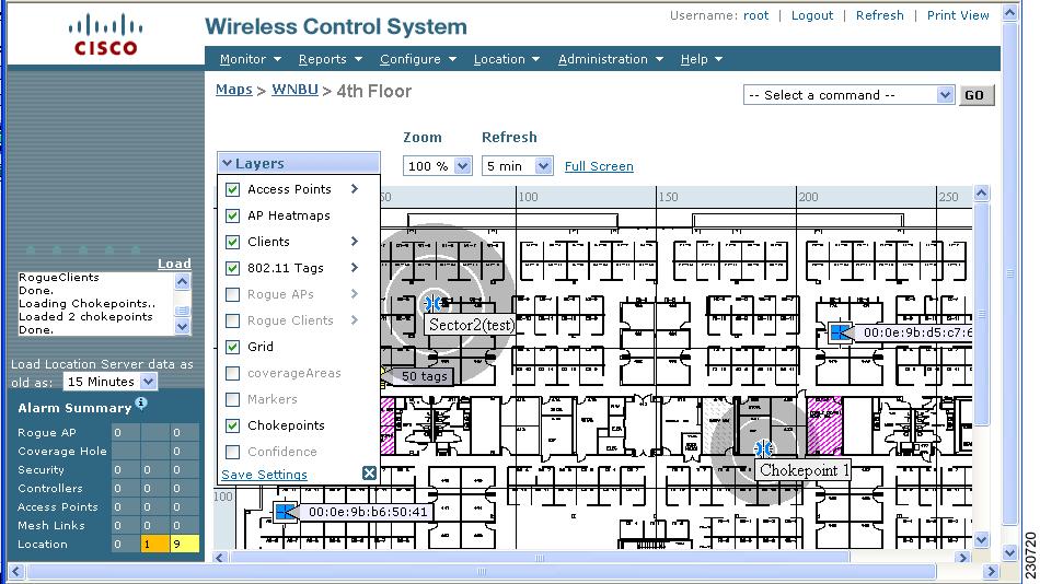
Step 1
Step 2
Step 3
•
•
•
•
•
•
•
•
•
•
•
•
Note
The enabled layers are checked, and the disabled ones are unavailable.
Note
Access Point Layer
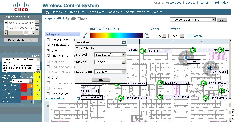
If you enable the Access Point layer and then click on the arrow to the right of these layers, an access point filter window appears with further menu options (see Figure 5-33).
Figure 5-33 AP Filter Window
Step 1
•
•
•
Step 2
•
•
•
•
•
•
•
•
•
•
Step 3
AP Mesh Info Layer
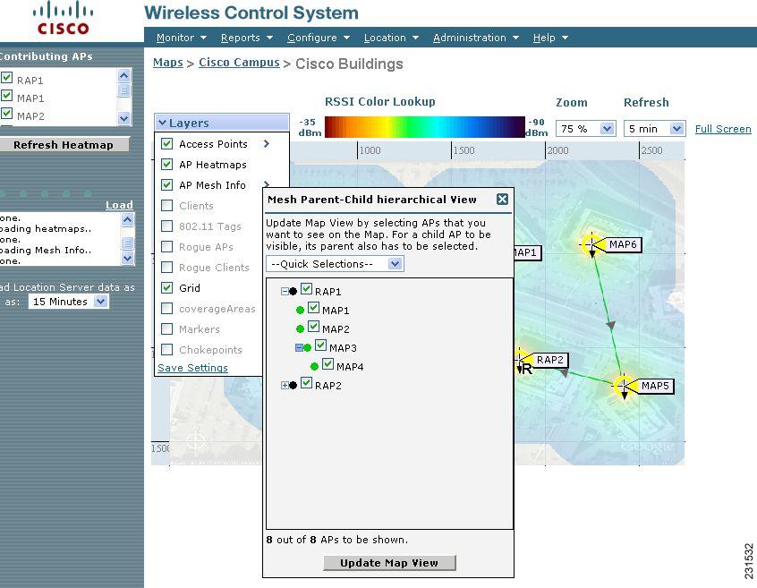
If you enable the AP Mesh Info layer and then click on the arrow to the right of these layers, a Mesh Parent-Child Hierarchical View window appears with further menu options (see Figure 5-34).
Figure 5-34 Mesh Parent-Child Hierarchical View Window
You can update the map view by choosing the access points you want to see on the map. From the Quick Selections drop-down menu, choose to select only root access point, various hops between the first and the fourth, or select all access points.
Note
Clients Layer
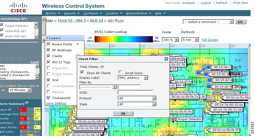
If you enable the Clients layer and then click on the arrow to the right of these layers, a Client Filter window appears with further menu options (see Figure 5-35).
Figure 5-35 Client Filter Window
If you click the Show All Clients check box and Small Icons check box, all other drop-down menu options are grayed out.
If you uncheck the Small Icons check box, you can choose if the want the label to display MAC address, IP address, user name, asset name, asset group, or asset category.
If you uncheck the Show All Clients check box, you can specify how you want the clients filtered and enter a particular SSID.
The Protocol drop-down menu options are as follows:
•
•
•
You can further choose to show clients in all states or specifically idle, authenticated, probing, or associated clients.
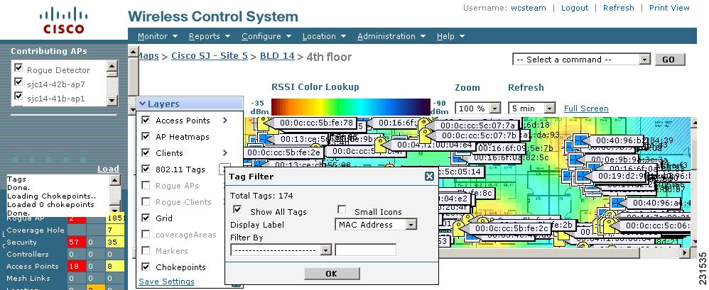
802.11 Tags Layer
If you enable the 802.11 Tags layer and then click on the arrow to the right of these layers, a Tag Filter window appears with further menu options (see Figure 5-36).
Figure 5-36 Tag Filter Window
If you click the Show All Tags check box and Small Icons check box, all other drop-down menu options are grayed out.
If you uncheck the Small Icons check box, you can choose if the want the label to display MAC address, asset name, asset group, or asset category.
If you uncheck the Show All Clients check box, you can specify how you want the clients filtered.
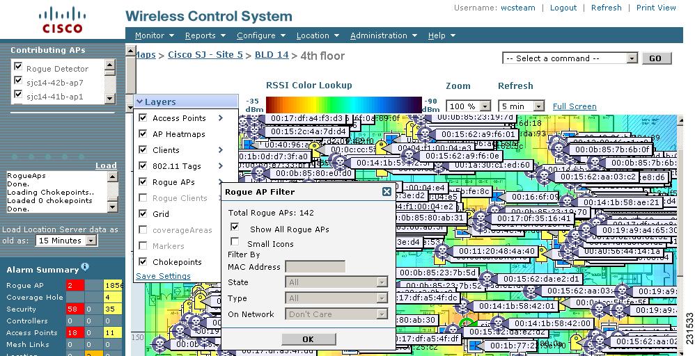
Rogue APs Layer
If you enable the Rogue APs layer and then click on the arrow to the right of these layers, a Rogue AP Filter window appears with further menu options (see Figure 5-37).
Figure 5-37 Rogue AP Filter Window
If you click the Show All Rogue APs check box and Small Icons check box, all other drop-down menu options are grayed out.
If you uncheck the Show All Rogue APs check box, you can specify how you want the rogue access points filtered. Follow these steps to define the filter.
Step 1
Step 2
Step 3
Step 4
Step 5
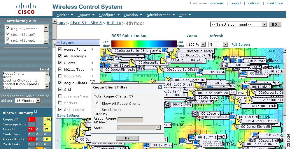
Rogue Clients Layer
If you enable the Rogue Clients layer and then click on the arrow to the right of these layers, a Rogue Client Filter window appears with further menu options (see Figure 5-38).
Figure 5-38 Rogue Client Filter Window
If you click the Show All Rogue Clients check box and Small Icons check box, all other drop-down menu options are grayed out.
If you uncheck the Show All Rogue Clients check box, you can specify how you want the rogue clients filtered. Follow these steps to define the filter.
Step 1
Step 2
Monitoring Channels on a Floor Map
Follow these steps to monitor channels on a floor map.
Step 1
Step 2
Step 3
Note
Step 4
Step 5
Step 6
The number of the channel being used by each radio appears in the flag next to each access point. "Unavailable" appears for disassociated access points.
Note
Monitoring Transmit Power Levels on a Floor Map
Follow these steps to monitor transmit power levels on a floor map.
Step 1
Step 2
Step 3
Note
Step 4
Step 5
Step 6
Step 7
Table 5-4 lists the transmit power level numbers and their corresponding power settings:
Table 5-4 Transmit Power Level Values
Level Number1
Maximum power allowed per country code setting
2
50% power
3
25% power
4
12.5 to 6.25% power
5
6.25 to 0.195% power
Note
Monitoring Coverage Holes on a Floor Map
Coverage holes are areas in which clients cannot receive a signal from the wireless network. When you deploy a wireless network, you must consider the cost of the initial network deployment and the percentage of coverage hole areas. A reasonable coverage hole criterion for launch is between 2 and 10 percent. This means that between two and ten test locations out of 100 random test locations might receive marginal service. After launch, Cisco Unified Wireless Network Solution radio resource management (RRM) identifies these coverage hole areas and reports them to the IT manager, who can fill holes based on user demand.
Follow these steps to monitor coverage holes on a floor map.
Step 1
Step 2
Step 3
Note
Step 4
Step 5
Step 6
The percentage of clients that have lost their connection to the wireless network appears in the flag next to each access point. "Unavailable" appears for disassociated access points, and "MonitorOnly" appears for access points in monitor-only mode.
Monitoring Clients on a Floor Map
Follow these steps to monitor client devices on a floor map.
Step 1
Step 2
Step 3
Note
Step 4
Step 5
Step 6
The number of client devices associated to each radio appears in the flag next to each access point. "Unavailable" appears for disassociated access points, and "MonitorOnly" appears for access points in monitor-only mode.
Step 7
Monitoring Outdoor Areas
Follow these steps to add outdoor areas to a campus.
Step 1
Step 2
Step 3
Step 4
Step 5
Step 6
Step 7
Step 8
Step 9
Step 10
Step 11
Step 12
Step 13
Step 14
Step 15
Note
Step 16
Importing or Exporting WLSE Map Data
When converting from autonomous to LWAPP and from WLSE to WCS, one of the conversion steps is to manually re-enter the access point-related information into WCS. This can be a time-consuming step. To speed up the process, you can export the information about access points from WLSE and import it into WCS.
Note
To map properties and import a tar file containing WLSE data using the WCS web interface, follow these steps. For more information on the WLSE data export functionality (WLSE version 2.15), go to http://<WLSE_IP_ADDRESS>:1741/debug/export/exportSite.jsp.
Step 1
Step 2
Step 3
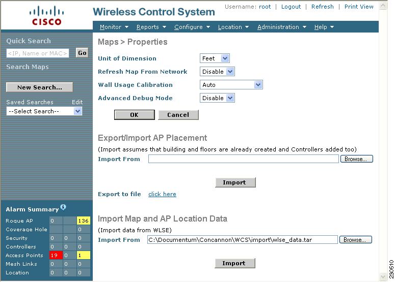
Step 4
WCS displays the name of the file in the Import From field (see Figure 5-39).
Figure 5-39 Maps > Properties Window
Step 5
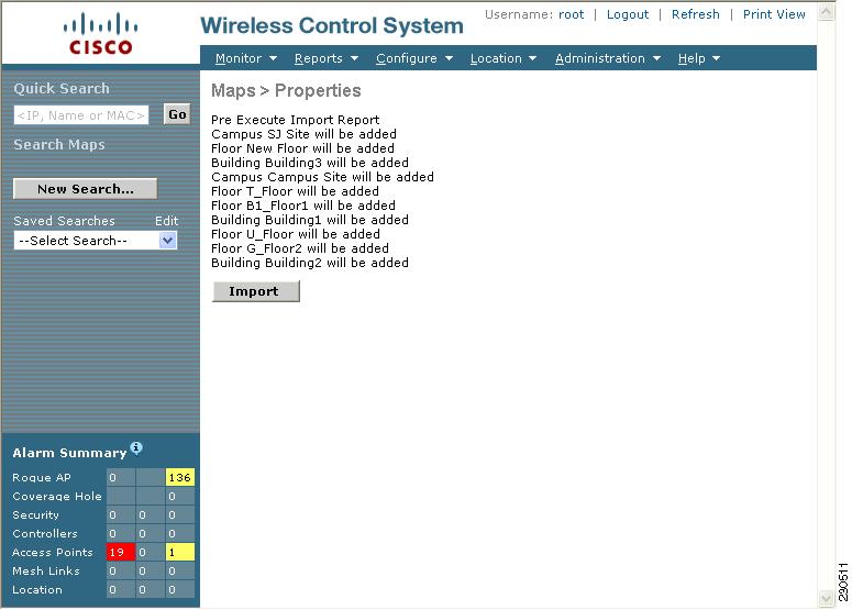
WCS uploads the file and temporarily saves it into a local directory while it is being processed. If the file contains data that cannot be processed, WCS prompts you to correct the problem and retry. After the file has been loaded, WCS displays a report of what will be added to WCS (see Figure 5-40). The report also specifies what cannot be added and why.
Figure 5-40 Pre Execute Import Report
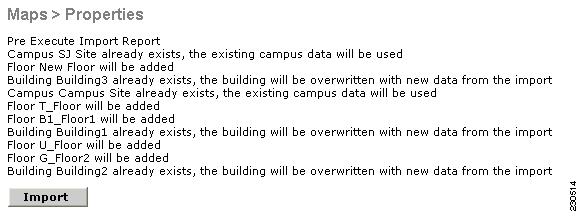
If some of the data to be imported already exists, WCS either uses the existing data in the case of campuses or overwrites the existing data using the imported data in the cases of buildings and floors (see Figure 5-41).
Figure 5-41 Pre Execute Import Report — Duplicate Data Handling
Note
Step 6
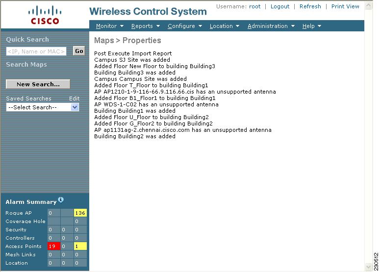
WCS displays a report indicating what was imported (see Figure 5-42).
Note
Figure 5-42 Post Execute Import Report
Step 7
Creating and Applying Calibration Models
If the provided RF models do not sufficiently characterize the floor layout, you can create a calibration model that is applied to the floor and better represents the attenuation characteristics of that floor. In environments in which many floors share common attenuation characteristics (such as in a library), one calibration model can be created and then applied to floors with the same physical layout and same deployment.
The calibration models are used as RF overlays with measured RF signal characteristics that can be applied to different floor areas. This enables the Cisco WLAN solution installation team to lay out one floor in a multi-floor area, use the RF calibration tool to measure, save the RF characteristics of that floor as a new calibration model, and apply that calibration model to all the other floors with the same physical layout.
You can collect data for a calibration using one of two methods:
•
•
Note
Use a laptop or other wireless device to open a browser to the WCS server and perform the calibration process.
Step 1
Step 2
Step 3
Step 4
Step 5
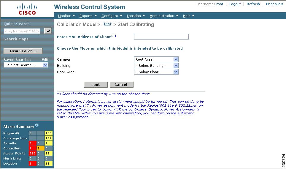
Step 6
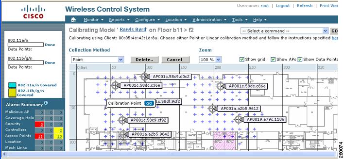
Figure 5-43 Starting to Calibrate
Step 7
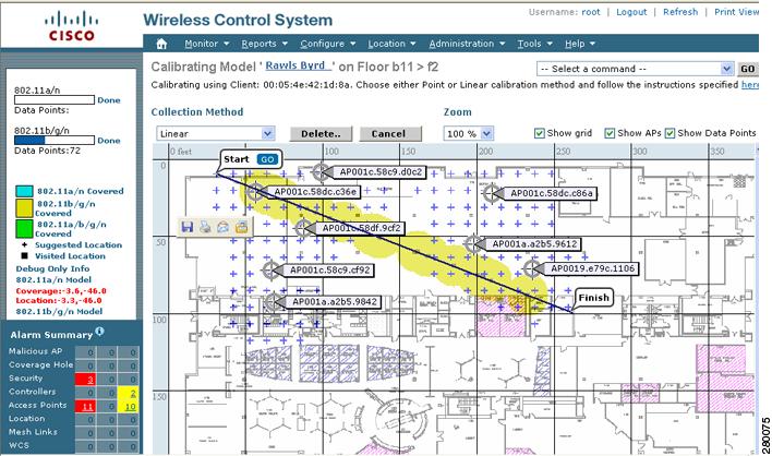
Using these locations as guidelines, you can perform either a point or linear collection of data by appropriate placement of either the Calibration Point pop-up (point) or the Start and Finish pop-ups (linear) that display on the map when the respective options are displayed. Figure 5-44 shows the starting window for a point calibration.
Figure 5-44 Positioning Calibration Points
a.
1.
2.
Note
3.
Note
Note
4.
Note
b.
1.
2.
3.
4.
Note
5.
Note
Figure 5-45 Linear Data Collection
Note
6.
Note
Step 8
Step 9
Step 10
Step 11
Step 12
Note
Analyzing Element Location Accuracy Using Testpoints
You can analyze the location accuracy of rogue and non-rogue clients and asset tags by entering testpoints on an area or floor map. You can use this feature to validate location information generated either automatically by access points or manually by calibration.
Note
Note
Note
Follow these steps to enable the advanced debug option and assign testpoints to a floor map to check location accuracy.
Step 1
Step 2
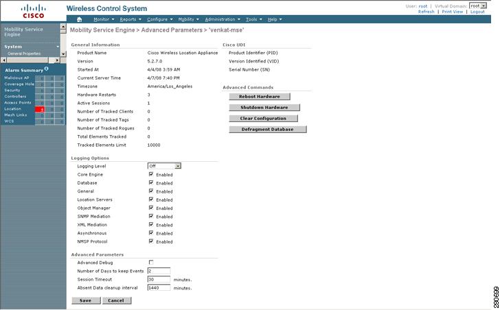
Step 3
Figure 5-46 Mobility Service Engine > Advanced Parameters
Step 4
Note
Assigning Testpoints to a Selected Area
You now must enable the Advanced debug level at the Maps level and begin assigning testpoints to a selected area or map.
Step 1
Step 2
Step 3
Figure 5-47 Map > Properties Page
You are returned to the Maps summary window. You are now ready to assign testpoints to a selected area or map.
Step 4
The page seen in Figure 5-48 appears.
Figure 5-48 Selected Area or Floor Map Chosen at Monitor > Maps Page
Step 5
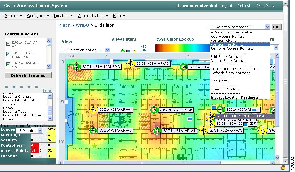
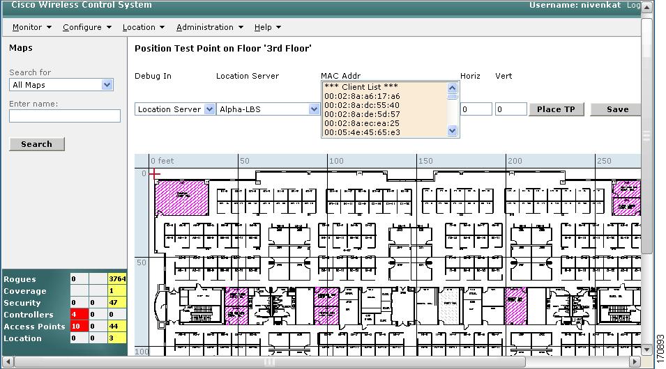
A blank map of the selected area or floor appears for testpoint assignment (see Figure 5-49).
Figure 5-49 Position TestPoint Assignment Page
Step 6
Note
Step 7
Note
A pop up box appears noting successful addition of the testpoint for the element and its MAC address.
The red cross hair cursor returns to the upper left-band corner after placement is confirmed. You are ready to mark additional testpoints.
Step 8
Note
Step 9
Step 10
A pop up window appears providing accuracy percentage and the number of sample points gathered during that interval.
You can perform this test for multiple elements by selecting multiple MAC addresses from the list of MAC addresses and repeating the above procedure.
Using the Accuracy Tool to Conduct Accuracy Testing
There are two methods of conducting location accuracy testing:
•
•
Both are configured and executed through a single window.
Note
Follow these steps to enable the advanced debug option in Cisco WCS.
Step 1
Step 2
Step 3
Note
You can now run location accuracy tests on the location appliance using the Accuracy Tool.
Using Scheduled Accuracy Testing to Verify Accuracy of Current Location
To configure a scheduled accuracy test, do the following:
Step 1
Step 2
Step 3
Step 4
Campus is configured as root area, by default. There is no need to change this setting.
Step 5
Step 6
Step 7
Note
Step 8
Note
Note
Step 9
Step 10
When you check a MAC address check box, two icons overlaying each other appear on the map.
One icon represents the actual location and the other the reported location.
Note
Step 11
Step 12
Step 13
Note
Step 14
Step 15
The Scheduled Location Accuracy Report includes the following information:
•
•
•
•
•
Using On-Demand Accuracy Testing to Test Location Accuracy
An on-demand accuracy test is run when elements are associated but not pre-positioned. On-demand testing allows you to test the location accuracy of clients and tags at a number of different locations. It is generally used to test the location accuracy for a small number of clients and tags.
Follow these steps to run an on-demand accuracy test.
Step 1
Step 2
Step 3
Step 4
Campus is configured as root area, by default. There is no need to change this setting.
Step 5
Step 6
Step 7
Step 8
Step 9
Step 10
Step 11
Step 12
Step 13
Step 14
Step 15
The On-demand Accuracy Report includes the following information:
•
•
•
Note
To do so, check the listed test check box and select either Download Logs or Download Logs for Last Run from the Select a command drop-down menu and click GO.
The Download Logs option downloads the logs for all accuracy tests for the selected test(s).
The Download Logs for Last Run option downloads logs for only the most recent test run for the selected test(s).